A Deeper Dive into Summary Levels
Summary Levels and Area Names
There are rigorously followed conventions for how the Bureau attaches names to geographic entities so that they can be readily identified. The name always describes the last entity for a hierarcical summary, sometimes followed by the notation "(part)". So here is what we get when we extract rows from the 2000 SF3 national ("B") file for the St. Louis metropolitan area:
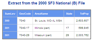
Notice the areaname values for the two 381 state portion summaries: you get the name of the state rather than the name of the metro area or a combination thereof. When viewed in context as it is here it makes pretty good sense. But when you work with the file and extract all the state-portion summaries and try to do analysis on them, it becomes a problem not having the name of the metro area on the records. Even when the MSA is contained entirely within a single state, the Areaname identifies the state rather than the metro area — we get "Texas (part)" instead of "Abilene, Texas Metropolitan Statistical Area".
Here is a listing of all the 390 level summaries on the Missouri "A" file:
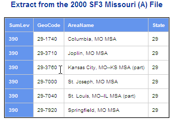
The names here are much more informative. They even use the parenthetical "(part)" notation to inform the user that the metro area spans states and this is only the part within Missouri. On the national file 381 summaries the word "(part)" is always appended, regardless of whether or not the MSA spans states.
Notice the GeoCode column shown in these extracts. This is not a Census Bureau field; it is one that the Missouri Census Data Center tries to add to most of our multi-summary level datasets. It contains the codes for all the fields that comprise the summary level, separated by by dashes. Thus the 381 level has 7040-29 for the Missouri portion of the St. Louis MSA, while the corresponding 390 level value is 29-7040.
Summary Levels by Size and Type
The summary level code for a place (the Bureau uses the the term "place" to mean an incorporated city or town, or a census designated place, which is a census-defined entity that has no legal definition but is used as a unit for data reporting) is 160. At least that is the code used on the 2000 SF3 files (per the Summary Level Sequence chart shown above). When the summary is for the portion of a place within a county the summary level code is 155.
So when the Bureau releases their "sub-county" population estimates, which include estimates for multiple geography types including places and minor civil divisions (county subdivisions that are legally recognized governmental units), they use summary level codes to identify the various levels summarized. Both complete place and place-within-county summaries are provided. You might expect to see these codes (155 and 160) used on these files. But here is what we get:
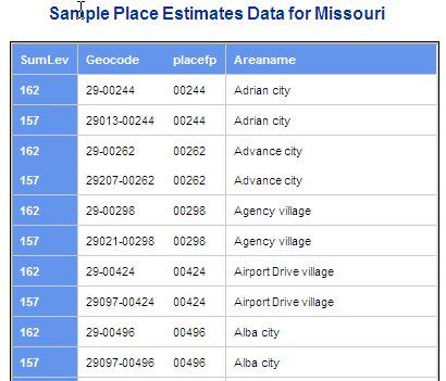
The expected 160 codes are 162s and the expected 155s are 157s. The explanation is that the Bureau uses a different code for these geographic units because the estimate do not include any CDPs (census designated places). A similar situation exists for the data estimated at the MCD level. MCDs are county subdivisions so you might expect 060 summary level codes. But instead you will see only 061 codes instead. These are a subset of the entities included within the 060 category.
This same thing happens when there is a geographic size limitation. In the 1990 national summary file they reported data at the place (city) level only for cities of at least 10,000 population. The summary level code used on those files was 161 rather than 160.
The moral of the story is that there may be more than one summary level code used to describe a geographic entity, depending on the context of where the summary data appears.
Historical Variations
The concept of a geographic summary level code has been around at least as long as the Census Bureau has been producing summary files (or "Counts" as they were called in the 1970 decennial census). For the 1970 and 1980 data products a 2-digit code was used. 01 was the code for a national total, 02 for a region, 03 for a division, 04 for a state and, you might expect, 05 might be a county. But actually 11 was the code for a county summary and all the rest are of no particular logical relationship to the new 3-digit codes that went into effect with the 1990 census products. Like a lot of historical facts, this does not have a lot of practical application. Unless maybe you happen to be required to go back and use some original census summary files from that earlier era. If you use data stored in the MCDC data archive, such as the stf803 and stf803x2 data directories ("filetypes"), you will see 3-digit SumLev variables that we created by converting the original 2-digit codes.
Metropolitan Areas
Metropolitan areas is an umbrella term that actually covers a number of different geographic entities. If you take the term as it has been used over time then there are numerous other entities that could be included. On the alternate chart we mentioned above, they have an entry labeled "core based statistical areas" instead of metropolitan areas. The CBSA terminology, used to describe a new system for defining these kinds or urban media-market type areas that was developed around 2000, has been discouraged by the Bureau and is not seen too often any more on their web site or in their documentation. A CBSA is either a metropolitan statistical area or a micropolitan statistical area, depending on the size of the core area. The CBSA entities were created as a replacement for the previous generation of comparable entities used from about 1982 through 2000, which were referred to as MSAs, CMSAs (Consolidated MSAs) and PMSAs (Primary MSAs). MSAs were simple stand-alone metro areas like St. Louis and Kansas City, while CMSA's were much larger urban entities that were made up of adjoining PMSAs. For example, the Dallas-Forth Worth, TX CMSA is comprised of the Dallas and Ft. Worth PMSAs). It was a little bit complicated and confusing and the CBSA's were an attempt to improve on the concept, especially by introducing the Micropolitan Statistical Areas which were just like the MSAs but on a smaller scale. Accompanying the new CBSA entities came two other related entities, Consolidated Statistical Areas (CSAs — combinations of adjoining CBSAs) and Metropolitan Divisions (sub-areas of CBSAs, which are roughly equivalent to the PMSAs of the earlier system).
While just trying to keep up with the various entities and the summarly levels and codes that go with them, there is also the variation over time which make using these geographic areas challenging. The CBSAs can and do change year by year. In most years the changes are rather few and somewhat small, but not always. You add a county here or there, occasionally (rarely) a county gets subtracted. New CBSAs can be created at any time during the decade and occasionally one gets decommissioned because it no longer meets the criteria. These changes do not draw much publicity and area easy to miss. OMB issues the formal bulletins that signal when changes occur. The Bureau then incorporates those changes into a text file with complete definitions (sometimes several months following the official OMB release).
The 2000 Census Summary File 3 Summary Level Sequence Chart
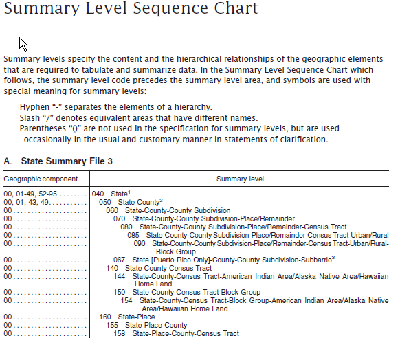
A familiar sight to anyone who has ventured into the field to Census Bureau technical documentation for their data prodicts (specificially, for the "Summary (Tape) File" products) is the document summarizing the geographic levels being summarized on these files. Here is a partial snapshot (only about a fourth of the entire 2-page document) of the Summary Level Sequence Chart provided with the 2000 Census SF3 data product.
Some things to note about the SLSC:
- The Geographic Component column alerts the user to the existence of special summaries that only consider a subpopulation of the area. For example a geographic component code of 01 indicates an "Urban portion" summary, 02 means an "Urban in centrl place of Urban Area" summary, etc. For most users all this means is that they are probably going to want to filter those rows where the value of the Geographic Component code is not 00 (the code indicating that is not a geographic component summary, but rather a summary of the entire geographic area.)
- The summary level codes and their meanings are indicated in the rightmost Summary level column. The first row entry of 040 State says we have state level summaries on this file indicated by a summary level code of 040. The second line indicates County level summaries with a code of 050. Note the indentation, which is crtitical to understanding these charts, as it indicates a hierarchy of entities. Counties are obviously nested within states. The footnote reference is provided to remind or inform the user that when we say "County," we include other entities that serve as county equivalents, such as parishes in Louisiana or boroughs in Alaska.
- Note the use of hyphens and slashes in the Summary level description, as explained above the table. In the row for level 070, for example, we have 3 dashes which means a 4-level hierarchy (starting with State and ending with Place/Remainder). The "/" in the last level says that this can either be a place (city or Census Designated Place) or it can be the "Remainder" of a county — the portion not within any place.
- The four codes 070, 080, 085, and 090 form a classic census geography hierarchy in which each level is subordinate to the previous one, all of them contained within the County Subdivision level. In Missouri a County Subdivision is called a "township" (in New England it is called a "town", and other names apply in other states). These levels are referred to as split (or hierarchal) geographies, i.e. as "split place" (070), "split tract" (080), and "split block group" (090). There are other summary levels (160, 140 and 150, appearing just below in the chart) which are the "un-split" summaries for these geographies.
- Being from Missouri, I have a certain bias regarding what summary levels are most useful and which ones we could almost get by without. Because it is rare for Missourians to care about township geography, there is not much interest in data tabulated to any of the gegraphies in the 070 to 090 hierarchy. These are very voluminous levels which typically can occupy a large majority of the space on a census summary file, and yet people in Missouri almost never care to use them. The exception to the rule is the 090 ("split block group") summaries. These are important summaries not because anyone cares about such data per se, but because they serve as building blocks when aggregating census data to other geographic levels. This is because these are the smallest geographic areas on Summary File 3, which means the smallest unit for long-form (aka "sample") data in the census. If you have only the 090 level summaries and the right programmer/software you can just about recreate through aggregation any of the component geographies (e.g. place, complete census tract, township, etc.).
- When people refer to "tract" and "block group" level data they are almost always referring to the un-split versions — summary levels 140 and 150, respectively. We (and the Census Bureau) refer to these un-slit levels as inventory levels and the split versions as hierarchal levels. This can somewhat explain why within the MCDC data archives you will sometimes see data files with names such as moi and moh. These contain inventory and hierarchal summaries, respectively. In 2000 there were 12,631 inventory summaries for Missouri and 30,172 hierarchal summaries. The moh dataset is 2.5 times larger than the moi dataset and about 1/10th as useful. See this page for a report indicating the SumLev variable values for the moh dataset and how often each occurs on the dataset.
Order Matters: Summary Levels 390 and 381 (for example)
If you follow the link just above to the complete summary level sequence chart for SF3, you will notice that it actually comprises two charts, labeled "A: State Summary File 3" and "B: National Summary File 3". Experienced census data users will recognized the Bureau's convention of release summary file products as a series of alpha-coded "files", such "Stf 3, File A" and "Stf 3, File B". The different files usually contain the same tabular data, but they do it for different geographic universes and summary units. In the case of the 2000 census, Summary File 3, there was a set of state-universe files that formed the "File A" series and a single national file ("File B") that presented data for mostly larger geographic areas but for the entire U.S.
On the second page of the A file SLSC you should see the entry:
390 State-Metropolitan Statistical Area/Consolidated Metropolitan Statistical Area
and on the second page of the B file SLSC the entry:
380 Metropolitan Statistical Area/Consolidated Metropolitan Statistical Area

  381 Metropolitan Statistical Area/Consolidated Metropolitan Statistical Area-State
You'll notice that the only difference between the description for the 390 and 381 summary levels is the order in which the component geographies are listed. On the A file State comes first, then the MSA/CMSA, while on the B file it is reversed. Of course we are really talking about the same kind of geographic entity — the state portion of metro area (which may or may not be in multiple states, by the way). It's not a signficant difference unless you think you know what the code is for such an entity and you try to plug the value in to your Dexter filter spec and have it fail because you are accessing the national file and using the state-file code. We have used this code-pair as an example of how this works. It also applies to other codes for geographic entities that can cross state lines such as Urbanized Areas, Core Based Statistical Areas and even ZIP (ZCTA) codes.