Data Allocation Using Geographic Equivalency Files
The Problem
A common problem encountered with using geography-based data (i.e. data that summarizes a set of geographic entities) is that we have data for some geographic areas describing a universe (such as a county or state) but not for some other sub-units of that same universe which are of interest. For example, we might have 2010 census data for units such as census tracts and block groups within a state, but not for the state legislative districts (house and senate) of that state. We shall refer to the units for which we have data as the source geography, and the units for which we would like to get data as the target geography. This terminology will be familiar to Geocorr users, where you get to choose two kinds of geographic layers from select lists labeled as Source and Target geographies. What we would like to be able to do is to process the data at the source geocode level to at least approximate data for the target units.
In this tutorial we want to focus on a few specific examples of doing source-to-target data allocations, outlining the basic algorithm and even pointing to some specific tools (in the form of SAS macros) that we have been using at the Missouri Census Data Center for more than 30 years. Our examples will make use of equivalency files (aka "correlation lists" or "crosswalk files") generated using Geocorr. We'll include discussions of how reliable the results may be and look at a way of measuring the reliability of an allocation.
We are not aware of any end-user-friendly applications that handle this allocation process. We assume that anyone wanting/needing to apply these methods will have some programming skills that will allow implementing the algorithm. We shall cite some SAS code because that is the language/resource we use for doing such processing. But obviously there are many other programming options.
The Solution (Overview of Process)
- Identify your source and target geographies, and the data to be allocated. The data must be available at the source geography level, and you must be able to correlate the source geographic entities to the target areas. Geocorr is a likely source for such a correlation, but there are many other possible sources. 30 years ago they were mostly created using base maps and clear plastic overlays.
- Extract the data at the source level and merge/join these data with the equivalency file, keying on the source geocode(s). It is vital that all source geocodes are associated with one or more target areas. When associated with more than one target area it is important to have an allocation factor to indicate what portion of the source area belongs to the target.
- Step 2 should result in a file that has target geocodes and allocation factors (usually), and the data to be allocated (describing the source area). This file gets sorted by the target codes and then gets aggregated to those units. A critical part of this step involves applying the allocation factors to the data prior to aggregating by the target areas.
- The result of Step 3 is aggregated to the target geocodes.
- Post-processing (optional) is done to assign various identifiers corresponding to the target gecodes. Assigning Areaname fields and geographic summary level codes, etc. This may not be an issue if the data are for personal use only, but if you are posting it to a public site it can be quite important.
Case Study 1: Block Group Data to Townships for a Single County
We chose this example because it was relatively uncomplicated and illustrates some of the issues you'll encounter doing allocations. It is not practical because the data we'll be allocating to the township ("county subdivision", called townships in Missouri) already exists. But that allows us to compare the approximations we'll be generating with the true values.
The problem statement:
For Adair County, Missouri we want to allocate a set of 10 basic demographic items from the 2010 census tabulated at the block group level to the county subdivision level (these are called "townships" in Missouri; it varies by state). There are 25 block groups and 10 townships in the county, which had a total population of 25,607 in the 2010 census. After doing the allocation we would like to do an evaluation step where we attempt to assign a reliability indicator to the output set indicating the extent to which the data for that area was allocated/disaggregated. We will also do a compare between our estimated results and the actual tabulations of the data from the 2010 census.
Generating the Equivalency File (using Geocorr)
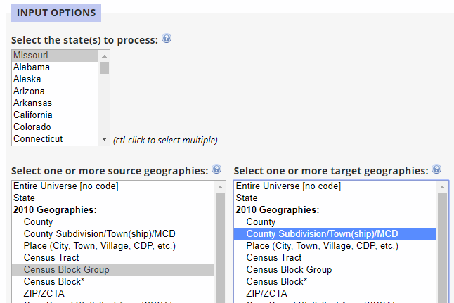
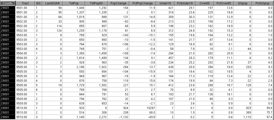
We choose "Missouri" as the state, "Census Block Group" as the source geocode, and "County Subdivision/Township/MCD" as the target geocode. We took defaults on most of the rest of the form options except that we entered "001" in the county codes box in the geographic filtering section of the form to limit processing to Adair county; and we chose to generate a second allocation factor, showing us what portion of the target's population was within the source. Here is the plain-text report generated by Geocorr:
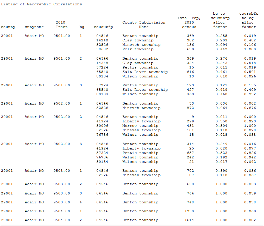
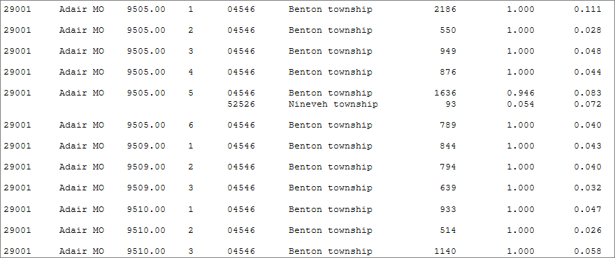
Does this look promising? Not great and not terrible. What we would like to see are a bunch of 1.000 allocation factors in the bg to cousubfp alloc factor column. Looking at the first block group (Tract 9501, BG 1) we see that it intersects with 4 townships. This means we'll be disaggregating the data for that block group to 4 areas. One of these, Nineveh, is a trivial piece, with just under 1%. Polk gets almost half of the BG (44%) while Benton and Clay get about 25 and 20%, respectively. We have similar cases for Tract 9501, BG's 2 and 3. These are the neighborhoods within the city of Kirksville. Note that once you get past tract 9502 you are in a much more rural area where the townships are larger and we see mostly 1.000 allocation factors in all these. That is a good thing since it means we can allocate all of those Block Groups to townships with no concern about the error that comes with disaggregation. What is that? It is the error that is introduced when we allocate data proportionally and assume/hope that the subareas are homogeneous. When we disaggregate the 9501/BG 1 data we give about 25% of all the BG data fields to Benton Township. In the case of Total Population, we know that this allocation is exactly right. But we also will allocate data items such as Persons Under 18 and Persons Over 65. Just because a quarter of the BG's total population is in Benton Township does not mean that the same portion of persons over 65 are as well. But that is the way we shall allocate, and that is where there is uncertainty (allocation error).
Get the Equivalency File Into Your Computing Environment
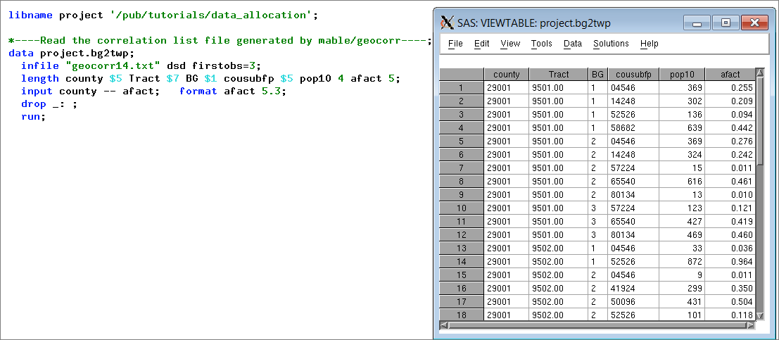
In our case, that means SAS. So we wrote a very short program to read the saved CSV file generated by Geocorr. Here we see that code next to a partial display of the resulting data set:
Create the Source Data Set: Data to be Allocated Tabulated at Source Level (Adair County BGs)
Here is the data we chose to allocate: three geographic ID fields and 10 numeric items for all block groups in Adair Co.
We pulled these data from one of our 2010 census SF1-based datasets with Missouri block-group-level data. We chose a dozen numeric variables for the purpose of illustration. We could have almost as easily pulled hundreds of variables, but we wanted to keep it simple so we could see all the data. Note that the geographic key fields — county, tract and bg — are in the same format as one on the equivalency file set. The LandSQMI variable is being rounded to the nearest integer in this display but actually contains fractional values that are typically less than 1.0 for the block group level.
Merge the Equivalency File and the Source Data Set to Create Aggregation Input
We have an equivalency file that has multiple observations (records) per source area (block group); at least for some of them. And we have a source data set with one and only one observation/record per block group. Both these inputs share the Adair county, MO universe. We shall do a one-to-many join of these two data sets. We use the following SAS code with a merge statement to handle the data-join logic:
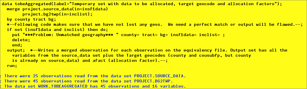
The SAS merge statement makes this pretty trivial. SQL users should have no problem coding the equivalent join. Note the code that checks to make sure there are no unmatched geographies. We need to match every block group on the source_data set with at least one observation on the equivalency data set. When there are multiple matches we'll have multiple output observations. The number of output observations should always match the number of observations on the input equivalency file.
The resulting data set (tobeaggregated) looks like this:
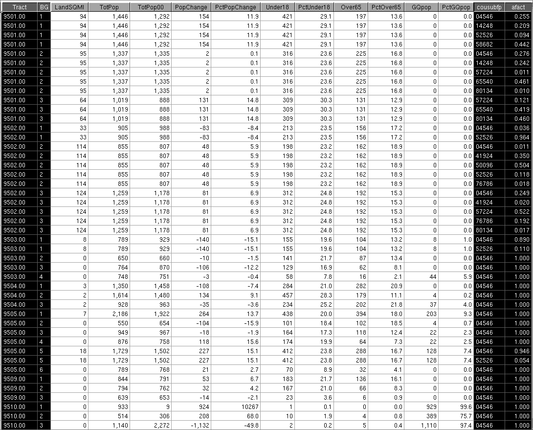
We have omitted the county from this display. It is a constant: 29001. Note how the township (cousubfp — county subdivision FIPS code) and afact (BG to township allocation factor, based on 2010 population) have been added. The LandSQMI field is being displayed as a whole integer, but the value actually stored is much finer and can handle values less than 1 with no problem.
Aggregating With Allocation
Now all that remains to do is to aggregate the data in this tobeaggregated data set by the target variable(s). The degree of difficulty here is dependent upon what tools are available to do the job. If you have to do it from scratch, without the aid of software tools that handle this type of processing, then you have some work to do. But if, like us, you have access to software that knows how to perform these tasks then the step becomes fairly simple.
Here is what we have to do to in this step:
- Sort the data to be aggregated by the target geocode variable(s) — in this case that is cousbufp. If we were not limiting our processing to a single county then we would need to use county and cousubfp.
- There are (in general) multiple observations for each of the target geocodes (in our particular example there are no instances of a target geocode (township) being associated with only a single source geocode (block group) — but this is unusual). We need to aggregate the data in these multiple observations (rows) to produce a single observation/row for each target geocode. If we did not have to deal with allocation factors, or with percentages the aggregation process would be very simple: just do the sums.
- To aggregate these data there are two things beyond simple addition that need to be done with the data. First is the application of the allocation factor to all the "summable" data items. By "summable" we mean that adding them together results in a value that makes sense in the aggregate. So variables such as TotPop and Under18 are summable. But PctChange and PctUnder18 are not.
- For the non-summable variables (all percentages in this example, but there are other kinds of items, such as population densities, per-capita income, average household income, etc. that would also fall into the non-summable category), we have to take weighted averages instead of simple sums. To do this we need to identify a weight variable corresponding to each of these percentages. The weight will be a measure of the denominator used in calculating the percentage. For example, the variable PctChange (measuring the percent change in population from 2000 to 2010) is derived as a percentatge of the 2000 population. So the weight variable for PopChange is TotPop00. For all the other percentage variables in this example, the weight variable is TotPop. (PctUnder18 is the percentage of the total population that is under the age of 18, etc.) To take a weighted average just means that you multiply the variable in question by the value of the corresponding weight variable, sum those weighted values and then in a post-aggregation step divide the sum of the weighted values by the sum of the weights to get the final weighted average.
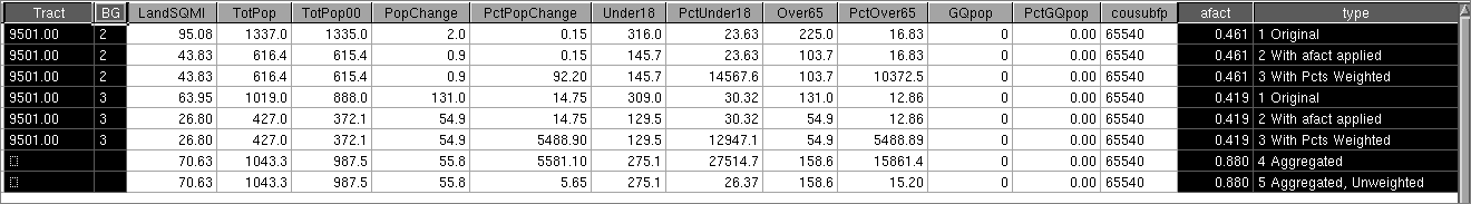
- For example, we have two observations on our sample tobeaggregated data set associated with target geocode 65540 (the code for Salt River Township in Adair County, MO). The following image shows some intermediate values representing the steps in the aggregation process where we look only at the two observations comprising the pieces we need to estimate the data for Salt River:
- Note the rightmost column where we have assigned a type value to indicate what the data in that row represent. For each of the two relevant input observations we see three type values: Type 1 is the orginal data to be allocated; Type 2 shows that data with the allocation factor value applied to all the "summable" (i.e. non-percentage) variables; Type 3 shows the observation with the percent variables weighted (and with the afact applied). Type 4 shows the results after we sum the values within the (2) Type 3 observations. Finally, Type 5 shows the final results, where we have divided the weighted percentages by the sum of the corresponding weight variable (TotPop in most cases) to get the final aggregate result.
The AGG Macro (SAS)
If you are a SAS user like us, we have a macro that can be used to implement the aggregation process as described above. Even if you are not a SAS user you may be able to borrow from the logic of this program to implement something comparable for other computing environments. We have online documentation for the macro, and the code itself.
Aggregating With the %agg Macro
Here is the SAS code we used to perform this aggregation process:
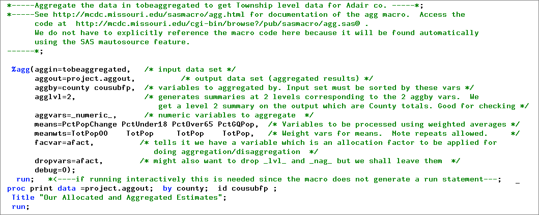
And here is the output from the Proc Print step to display our results:
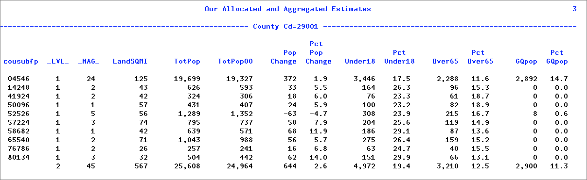
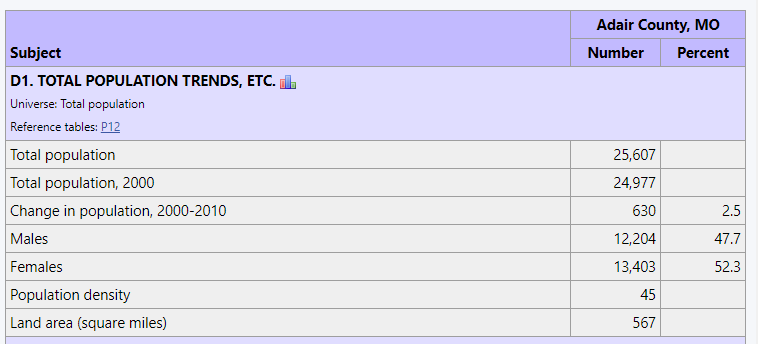
How did we do? A good first step in verifying the results is to look at the last observation here, the Adair county totals. These values are readily available from various sources including the MCDC's 2010 Census SF1 Profile Report application. When we run that app for Adair County, we get a report that includes:
and
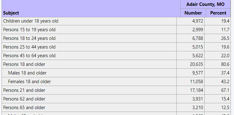
When you compare the numbers in our allocated data set with these what do you see? They match almost exactly. Or at least the total population, the persons under 18 and over 65 are exact. The 2000 population estimate differs by 13 (out of almost 25,000) and would be exact except for roundoff issues at the block group level. Not shown here, but also an exact match is the group quarters population, as is the land area in square miles.
So does this mean our allocations are "perfect"? Not at all. It just means we probably do not have any processing errors. When we do our allocations all we do is chop our block group data into smaller pieces representing their intersections with townships. The "error" (i.e., the difference between our estimate and the true value) occurs at the township level. But all these smaller pieces still add up to the BG values, so when we do our aggregation it makes perfect mathematical sense that all the BG pieces should sum up exactly to the county totals. But what about at the township level?
To help us get a handle on this question we did some custom processing of the data, comparing the results of our allocation with the township level actual data from the 2010 census. We created a data set with four rows per township. The type variable indicates the meaning of each row. Here is the resulting report that shows us how we did with our estimates.
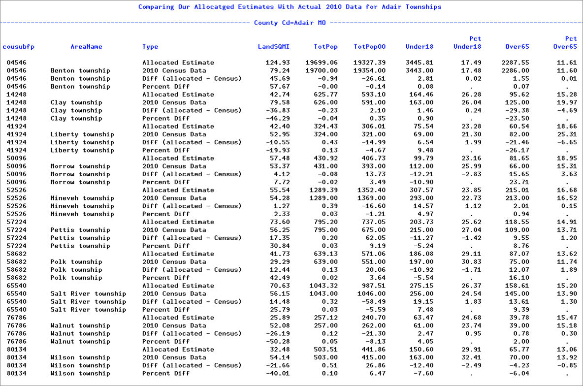
We omitted the GQPop and PopChange variables from the report. Some things to notice on this report include the following:
- The LandSQMI estimates are really way off. Not surprising if you think about it. We were allocating land area under the assumption that it was proportional to population, and that is simply not the case. In fact, smaller populations tend to indicate more rural area and these are typically larger. The moral here is that when using population-based allocation factors restrict the variables to those linked to population. The ideal allocation would be done in multiple parts using multiple allocation factors. For example, you might want to allocate housing data using housing count as the basis of the allocation factors (available option in Geocorr), and population-based allocation factors for person data. But at least population and households are closely correlated, so using pop-based factors for housing unit data still works pretty well.
- The Benton Township data is very good. This is because it's a very large township (having around 80% of the county's total population). This is generally true — estimates are better for larger target areas and worse for smaller ones.
- The estimates for the younger 0-17 age cohort were better (no township was off by more than 10%) while for the seniors there were a number of cases where we were off by more than 10%. One reason for this is that the numbers are larger for the younger cohort.
- Overall I would say the allocation was good, but not great. Maybe a B-. It gets a lot of things right and a few things — especially smaller subpopulations for smaller geographic areas — not so good.
- Adair county is a tough case because of the small townships. We would do better using a more urban/suburban county.
- The Areaname variable is blank on the "Allocated data" rows, but then appears on the rest (comes from the SF1 census data). In a typical data allocation process, you will need to have a final post-processing step where you add identifiers to your new data, and one of these is usually a name for the areas. Where such names come from depends on the target geography.
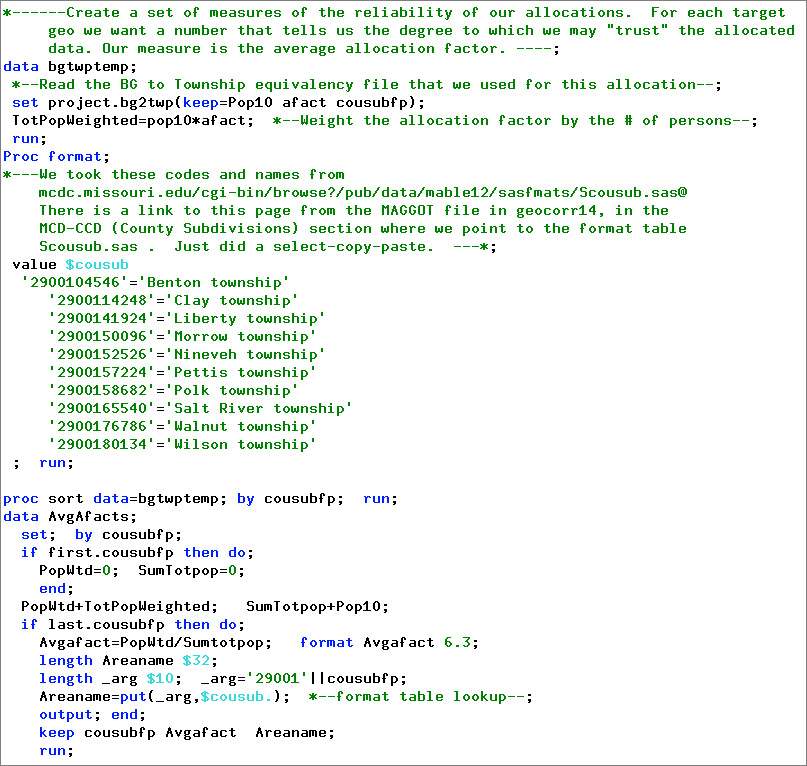
Defining an Average Allocation Factor
We have said that allocations are more reliable for larger areas, and less so for smaller ones. But is there a way we can actually create a measure of the reliability of the data allocated to a specific geography. The uncertainty comes when we have to allocate (i.e., when the afact variable has a value other than 1.0) data. If an area is the result of taking 20% of geocode A and 30% of geocode B, vs. an area where we took 100% of C and 90% of D, which would be the better estimate? Clearly, the latter case yields a more reliable result because we are doing less allocation. And we can easily measure this characteristic by simply taking the weighted average of the allocation factors in our correlation list, weighting by the population figure used to create the allocation factor. We did this with the correlation list used in this case study and got the following results:
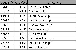
As we thought, Benton is by far the "best", while Walnut township comes in last. The factors tend to be correlated with size in this case. Here is the SAS code we used to generate these data (the above is just a viewtable display of the AvgAfacts data set):
Case Study 2: Allocating Census Data Across Decades
The first case study was a teaching tool where we kept things very simple so we could focus on the mechanics of doing an allocation. In this second case study, we'll be looking at a real world application that we actually coded and ran here at the Missouri Census Data Center. The problems we address here are not at all uncommon with census data for small geographic areas. The best units for small area data analysis of census data are census tracts and block groups. One of the bad things about these units is that they are redefined every ten years, so to get trends you have to figure out a way to get the "old" (previous decade) data into the "new" (current decade) geographic entities.
In the very important case of the American Community Survey (ACS) data, we have an interesting opportunity/challenge regarding census-tract-level data. We would like to look at trends in ACS data for census tracts in calendar year 2016, when the available ACS data vintage was 2014. We are warned against using overlapping 5-year intervals to do trend analysis. However, the earliest 5-year data available (2005-2009) does not overlap with the 2010-2014 data. The bad news is that back in 2010 when they were creating the 2009 vintage data, they were still using the old census 2000 geography for block groups and census tracts. What we want to do is take the 2005-2009 data, tabulated to 2000 census tracts, and do an allocation of those data to get them into 2010 census tracts, so that we can compare them with the vintage 2014 data.
Getting the Equivalency File from blkrel10
To do this allocation we are going to need an equivalency file relating the 2000 census tracts to 2010 census tracts. Since we are going to be allocating ACS data for 2005-2009, we would like to have allocation factors based on the population of the intersections in the latter part of that time period. That would be ideal. But, we really do not have any publicly available data at small enough geographic units to create an equivalency file based on (say) 2007 estimates. But a list based on 2000 population counts would be pretty good, if not ideal. It turns out that is what we do have, and that is what we shall use. Can we get such a list using Geocorr? The answer is "no" — Geocorr unfortunately does not provide small-area links across time. So, we need to look for another source.
As you would expect, the Census Bureau does provide tools for linking 2000 census blocks to 2010 blocks. They are called block relationship files — see the Bureau's Relationship Files web page. They even have tract relationship files, but we only processed the block relationship files. We were then able to easily create tract-to-tract equivalencies from the block-to-block data. We stored these data in the blkrel10 data directory of our public data archive. To get a true population-based 2000 to 2010 block equivalency file, we would need to know how many people lived in each block intersection. We do not have that, but what we do have is the size of the spatial intersection of these blocks. We then disaggregated the 2000 population of the 2000 blocks to 2010 blocks based on the spatial measure. If 2000 block A had 50% of its area within 2010 block B, then we estimated the population of that intersection to be .500 of the 2000 population. While that is not a particularly reliable assumption, keep in mind that most uses of the derived equivalency files will be for much larger areas, where the entire 2000 block is contained within the target area, so that the block allocation factors do not matter. For people who read SAS code and want to get down to the nitty gritty, you can see the code we used to process these block relationship files in the Tools subdirectory of the blkrel10 data directory, file blkrel2010.sas. In this program, we create a set of state-based block-to-block relationship files and then a set of corresponding tract-to-tract files. Here is some of the code used:
***Step G***;

*---create a block 2k to block 2010 correlation list (equivalency file)----;

%corrwt(setin=blkrel10.&stab.blks,geocds1=state2k cnty2k tract2k blk2k, geocds2=state cnty tract blk, wtvar=Pop2kInt, keepwt=1, afacts=1, exitout=xcode, setout=blkrel10.&stab.bl2k_bl10);

***Step H***;

*---create a tract2k to tract10 correlation list (equivalency file)----;

%corrwt(setin=blkrel10.&stab.blks,geocds1=state2k cnty2k tract2k, geocds2=state cnty tract, wtvar=Pop2kInt, keepwt=1, afacts=1, exitout=xcode, setout=blkrel10.&stab.tr2k_tr10);

run;
The corrwt macro does most of the work here. This is the macro that the Geocorr web modules invoke to do the heart of the geography processing. The geocds1 parameter specifies the source geocodes, while geocds2 is the target list. The appearance of &stab. in the setin/setout parameters tells you that this code processes data for a specific state whose postal abbreviation is stored in global macro variable stab. We have a utility macro called %dostates that we use to invoke a state-based processing macro to repeat that code for either all or selected states in the US.
Handling MOEs
In this real-world application, things are a bit messier. For example, we do not have just 10 numeric variables to aggregate. We have hundreds of variables. Almost half of these are percentages (if there is a variable called Age0_4 you can just about bet on there being a variable called PctAge0_4). There are also variables that contain margin of error values (MOEs). We opt to not process these variables, but we need to get a list of them so we can specify that they be dropped. We could do it without using special tools to help, but that would be not only very tedious and time consuming but could also affect the reliability of the results.
Handling Medians
Some of the most commonly used ACS data items are medians. Median age, median household income, median home value, etc. are all key indicators. But the data we shall be using on input is a special extract done using more detailed data from the complete set of summary (base) tables provided. We have 11 medians in our standard profile data sets. Of these 11, four of them have other variables that form a distribution table corresponding to that median. For example MedianHHInc (median household income) can be paired with the ten variables HHInc0, HInc10, ..., HHInc200 that form a distribution table from which a median could be estimated. But the ten intervals are a significant collapsing of the 16 intervals on the more detailed distribution in the base tables. This means that even if we were to make the extra effort to estimate the median by a post-aggregation step where we used data from the aggregated distribution, it would not be all that accurate because of the lack of detail. The same situation applies in each of the four cases where we had some distribution figures. So what we do instead is violate the statistician's code and estimate the median values by taking their weighted averages. The result is a weighted average of the medians of the components, but it is not the median of the aggregate. It may not be the actual median, but it is still a not bad measure of the typical, middle value of the distribution.
Handling Means, Percentages, Ratios, etc.
A common problem when doing aggregation is to make sure that variables that are not not directly aggregatable get aggregated properly. It is easy to aggregate variable HvalOverMillion (number of homes with value of $1,000,000 or more) but what about PctHvalOverMillion? If you had to aggregate four observations to get an output record you cannot simply add up the four percentage values and get a result that makes any sense. What you really have to do is recalculate the percentage by aggregating numerators and denominators and then recalculating the percentage following the initial aggregation. This turns out to be equivalent to taking the weighted average of the percent variables, where the weight variable is the denominator used in calculating the percentage. In the case of our PctHvalOverMillion, the denominator is OwnerOcc — number of owner-occupied housing units. Taking weighted averages also works for variables like PCI (per capita income, which is just an average) or AvgFamilyInc. So how does one calculate a weighted average? Simply:
- To take the weighted average of variable P using weight variable W, multiply P by W prior to the actual aggregation (summing).
- Aggregate the data.
- In a post-aggregation step, divide the total of the weighted P values by the total of the W values. This is the weighted average of P.
Dealing With Imperfect Geographic Data
One of the uglier real-world realities that needs to be dealt with in doing this processing has to do with making sure that the geographic codes that are used on our equivalency file (based on the blkrel10 data sets) match up with those being used in the ACS data. There are four geocodes being used here: the 2000 vintage county and census tract, and the 2010 versions of the same. So why should we have to worry about our codes all matching up? They all come from the same source (the Census Bureau), and that source is known for its reliability and attention to geographic detail. So what could go wrong? Here is an example, extracted from the Bureau's 2009 Geography Changes page:
"There are major changes to the geographic definitions for two of the Census 2000 tracts in Ketchikan Gateway Borough and Prince of Wales-Hyder Census Area, resulting from the substantial annexation of territory by Ketchikan Gateway Borough from the former Prince of Wales-Outer Ketchikan Census Area. However, the remaining Census 2000 tract definitions in these areas are unchanged. The following describes the comparability of Census 2000 tract definitions in the current context, compared to their original definitions in Census 2000.
"Tracts 1, 2 and 4 in Prince of Wales-Hyder Census Area have the same definitions as Tracts 1, 2 and 4 in the former Prince of Wales-Outer Ketchikan Census Area from Census 2000.
"There are substantial changes in the geographic definition of Tract 3 in Prince of Wales-Hyder Census Area, and there is no comparability with Tract 3 in the former Prince of Wales-Outer Ketchikan Census Area from Census 2000. Tracts 2, 3, and 4 in Ketchikan Gateway Borough retain the same Census 2000 tract definitions.
"There are substantial changes in the geographic definition of Tract 1 in Ketchikan Gateway Borough, and there is no comparability with the original Census 2000 definition of Tract 1 in Ketchikan Gateway Borough.
"Lastly, AFF access to ACS 5-year estimates for Tracts 1, 2, 3, and 4 in the former Prince of Wales - Outer Ketchikan Census Area are accessed through the successor Prince of Wales-Hyder Census Area instead."
The changes for the 2000 census tracts were confined to the states of Alaska (worst case), Colorado (the creation of a new county, Bloomfield, created problems), and Clifton Forge, VA. These are the valid changes. But then you should read the final section on this changes page. The first paragraph of this section explains:
"Census tracts and block groups used to tabulate and present 2005-2009 ACS 5-year estimates are those defined for Census 2000. However, in 19 counties from 8 different states, many of the census tracts and block groups used to tabulate and present the 2005-2009 ACS 5-year estimates are either those submitted to the Census Bureau for the 2010 Census, or a preliminary version of 2010 Census definitions. These census tracts and block groups were inadvertently included in the version of the Census Bureau's geographic database (TIGER) used to produce geographic area information for the 2005-2009 ACS 5-year estimates."
The only good news here is that the problem is well documented. (The Census Bureau does not always correct their mistakes, they just document them.) There are good and precise descriptions of what happened during the years following 2000 in Alaska, Colorado and Virginia to cause significant restructuring of the census tracts used for tabulating the 2000 census. So why is this relevant to our allocation project? Because in the blkrel10 files released circa 2001 the county and tract codes used are the original as-of-the-2000-census codes. But the codes that the Bureau uses to tabulate the tract-level data for the 2005-2009 5-year estimates are those reflecting the valid changes and mistakes described above. This means when we do that potentially simple step of joining/merging the equivalency file (blkrel10) with the source data (acs2009), we are not going to have a perfect match — not unless we first engage in the tedious task of translating the above narrative descriptions of what changed into a block-level file telling us what the "new" county and tract codes are whenever they do not match what they were at the time of the 2000 census. We have done something like this dealing with similar changes to the 2010 census tracts vs. the ones currently being used in the 2014 vintage ACS data. It took us several days to write the code to capture those changes at the block level. And we have not even talked about how to deal with the problems with the wrong tracts used in the 2005-2009 ACS data. They provide spreadsheets to help with seeing the problems, but admit that there are some cases where it will not be possible to overcome the errors and get data by the original 2000 tract geographies, per this excerpt from their description of the problem:
"The purpose of inclusion is to identify the tracts and block groups where this condition is true, and acknowledge that in some cases comparisons to Census 2000 tracts and block groups is not possible."
There are actually two sets of geographic fixes required to make our results be what we want. We need to get updated 2k tracts on our equivalency file so that they will match the tracts used on the 2009 vintage ACS files. But we also need to update the 2010 tracts as well. If we do not then the output data set will not reflect the current tract-level geography being used on the 2014 ACS data. And the whole point of doing this allocation is to get something that we can match up with the 2014 data and look at trends. The task is easier on this side because there have not been as many changes this decade as there were in the previous one, and because we have already done some work on creating a data set that will help us with these updates.
So, how are we going to handle this? We are going to take a cue from the Census Bureau, for the time being: Document the problem, but don't fix it. The errors will occur during the step where we join our equivalency files with our 2005-2009 ACS data. We match using the key variables county and tract, as of 2000. The problems will occur in places where the 2000 tract has had to revised (only affects 3 states: AK, CO, and VA, as noted above) and in states where the Bureau used post-2000 tracts for tabulating the 2005-2009 data. As we do our join/merge, we can document mismatch problems to identify cases where the 2000 county/tract on the block relationship file does not match the county/tract codes on the vintage 2009 ACS data. We can afford to take this somewhat cavalier position, since our most frequently used states — Missouri, Illinois, and Kansas — are not affected.
Allocate2trk2010.sas — the Program
We at the Missouri Census Data Center maintain a public archive of data, most but not all based on data from the Census Bureau. We also provide special web applications to allow users to access and query these data. If you are not familiar with our Uexplore and Dexter applications you might want to follow the link in our blue navigation box to the data archive home page, which has lots of links to both the software and to sections of the data archive (categories we call filetypes). One of the filetypes we have is called acs2009 and has data based on the vintage 2009 American Community Survey data. With that directory, we already have a data set containing the 5-year period estimates at the census tract level. This is not a tutorial on how to access our data archive, so we are not going to get into great detail here. But one of the data sets that we have in this collection is a standard extract of more than 300 key data items each of more than 170,000 geographic areas covering the entire U.S. Among those geographic areas there are more than 65,000 at the census tract level. These entities are the 2000 census tracts. These are the data we'll be using as our source. We shall be allocating and aggregating these data to get estimates of these data items at the 2010 census tract level.
The result of this data allocation shall be stored in the public data archive as well, in the same directory — acs2009. We'll also be making the code used to create that dataset accessible as well.
State-by-State Strategy
We could do this all in one huge step where we read in data for the entire country and then wrote just a single output data set with data for the entire country, similar to the input data set. But we choose not to. Instead we shall do these state by state. It is a bit easier to code that way, and it allows us to bypass states where there might be data problems. We have a simple coding strategy that employ for most of our national data collections. We write code to process a single state in the form of a SAS macro that has a standard interface with two positional parameters called state and stab. The first contains the 2-digit FIPs state code (with leading zeroes), while stab contains the 2-character state postal abbreviation. Within the macro we reference these parameters rather than specific values. To specify the state whose data we want to extract from the usmcdcprofiles5yr data set, we code [where] state="&state" (as opposed to the more straightforward state="29"). Once we get the code working, we can then invoke the macro to do selected states (especially valuable while debugging) or we can easily invoke it for all 51 states using our %dostates utility macro.
Generating Variable Lists
We have three lists of variables that we shall use for our conversion processing. We need a list of all the variables that are margin-of-error values, so that we can specify that we want these dropped from the input data step. This could be coded manually but it would be very tedious and error prone. Fortunately, it is pretty easy to do this by combining our strict variable naming conventions with a sas utility macro. All such variables have names of the form {variable-name}_moe, where {variable_name} specifies the name of the variable for whuch this is the corresponding MOE measure. Our utility macro, %varlist (written by David Ward), allows us to specify a data set and a name pattern such as "*_moe" and have it return a blank-separated list of all variables on that data set with names matching the pattern. We code this as
%let moes=%varlist(*_moe,acs2009.usmcdcprofiles5yr);
The list of more than 340 MOE variables can now be referenced when needed in our program by just coding a reference to &moes.
The other key variable lists we need to save us from tedious and error prone coding are the lists of mean variables and the corresponding mean weights that can be used to weight those variables when doing aggregations. Fortunately we have a metadata data set where we keep such information regarding the variables in our mcdcprofiles-type data set. This is the data _null_; step beginning around line 30 of the SAS program file. This step creates two global macro variables named means and meanwts, and the values of these variables are the lists we shall need to tell %agg how to handle these variables. There are 330 such variables, which include all of the Pct variables. In addition to creating this pair of global macro variables, the step also writes a file with a short report showing how the means and their weight variables pair up. This report can be viewed in the meanwts.txt file in the same Tools directory as the conversion program.
Processing the Source ACS Data
Now that we have finished defining some key variable list macro variables we are ready to begin the actual processing of the data. We begin (circa line 70 of the program — note that we are inside the %doit macro) with a data step that defines the acstracts data. Here is the SAS code that accesses the ACS data to be aggregated/allocated and then merges it with the tract 2000 to tract 2010 equivalency file to create the data set with 2010 tracts ready to be aggregated.
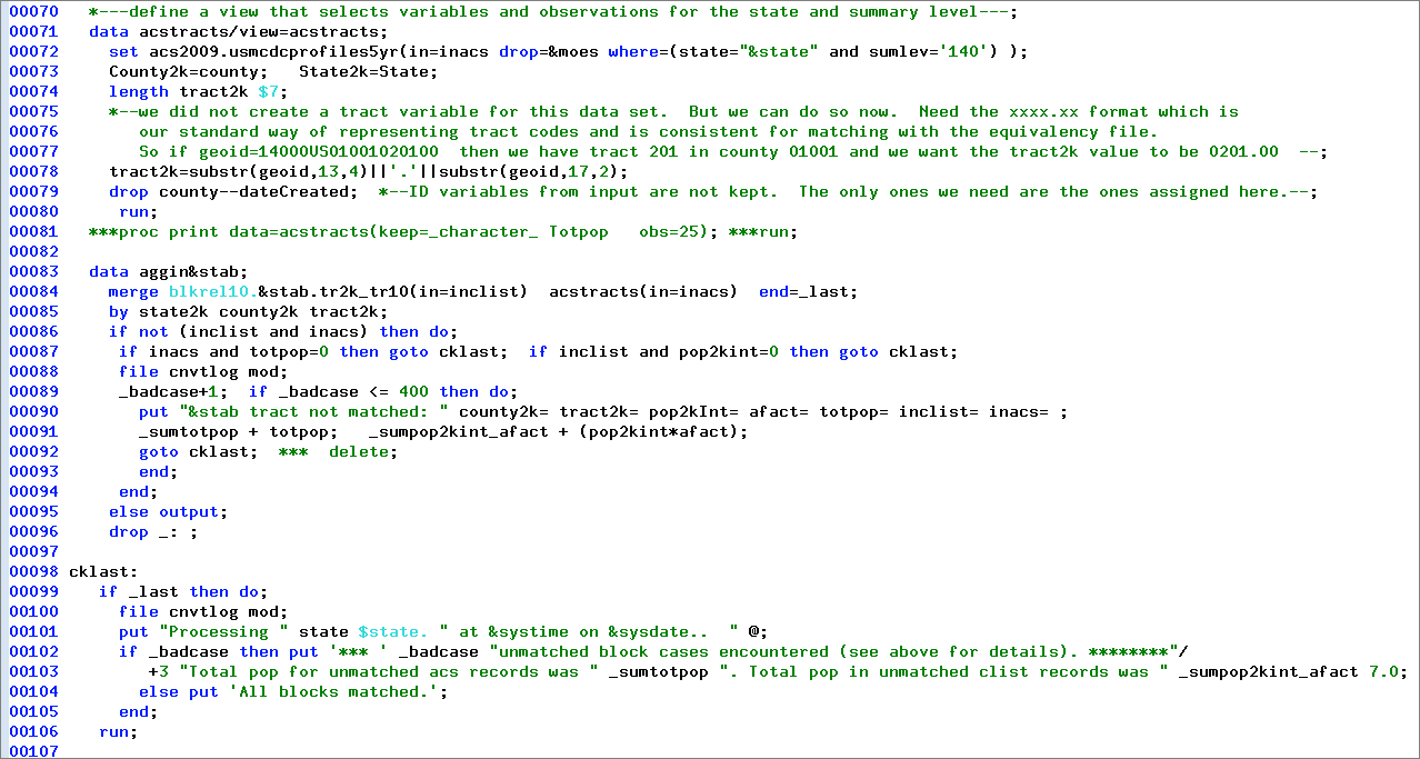
The key statement here is the set statement at line 72 referencing the very large acs2009.usmcdcprofiles5yr data set:
set acs2009.usmcdcprofiles5yr(in=inacs drop=&moes where=(state="&state" and sumlev='140') );
The set statement is used to read SAS data sets, one observation at a time. The drop=&moes specification tells SAS not to bother with all those variables that have names ending in _MOE. The where clause — where=(state="&state" and sumlev='140') — specifies the conditions for having an observation actually read during the data step. It specifies that we only want those observations where the value of the variable state is equal to the value &state — the value we specify as the first positional parameter when invoking the %doit macro. If we are processing Missouri, this turns into state="29".
The second condition (which is connected to the first with the and operator, meaning we want both conditions to be true) specifies that we only want those observations where the value of variable sumlev is 140. Census data geeks will recognize this as meaning we want summaries at the census tract level. Ignore all those other state, county, place, ZCTA, PUMA, etc. summaries — we only want complete census tracts. When we run the macro for Missouri it will pull out just over 1900 observations (cases, tracts, ...) from the more than 170,000 on the complete referenced data set — and will do this in a matter of a second or less because the input set is indexed by state.
Processing the ACS Source Data and the Tract-to-Tract Equivalency
The data step beginning at line 83 (data agiin&stab;) is the key to doing the allocation. This is the step where we merge (i.e. combine, join) the ACS estimates data with the equivalency file. The SAS merge statement takes care of the program logic for doing the join. Using in= variables, it is easy to know what you are dealing with in terms of the two files being matched for a given cycle of the data step. It makes it easy to know when you have a case where one of the two data sets is not matched. The by statement (line 85) specifies the variables used to link the observations from the two data sets. We have a one-to-many merge here: there can be multiple observations on the blkrel10 equivalency file with the same by variable keys (identifying a 2000 census tract), but there should be only (at most) a single observation with these by variables on the acstracts data set. Each time we have a match an observation is written to the output data set (aggin&stab). The if statement at line 86 checks to see if we have a match, i.e. if both of the in= special flag variables as specified on line 84 are set to true to indicate we have a case where both input data sets are contributing. If we have a tract that is in the data but not in the equivalency file, then we do not know where the allocated values are to go, and if we have an equivalency file tract without any matching ACS data, we have no data to allocate. So we really need to have only cases where the tracts match between the data and the equivalency file. When they do not match it is an error that needs to be looked into to avoid invalid output. The code at lines 87 to 94 are error handling. We opt to ignore cases where we have a tract with 0 population (it does happen), and also if we have a case where the equivalency file indicates a zero population intersection. The "bad" case gets documented on the cnvtlog file where we keep track of these problems. This file is the same no matter what state is being processed and gets written to mod, meaning when we start processing Alaska we just pick up from what we wrote to this file while processing Alabama. It becomes a rather important file, because it lets us know which states are going to need some work before we can fully trust the allocated data for them. The other key thing to note in this error handling block is the goto cklast; statement at the end of the do group. Turns out that we do not really need that statement, but it emphasizes that we do not want to output to aggin when we have a problem case. The statement is not needed because we modified line 95 to specify that the output statement (which is what causes the program to actually write something to the output data set) will only be executed when the condition at line 86 is false, i.e. when we have data from both input sets.
Note that we can easily detect when we are finished processing using the end=_last spec on the merge statement. When we are processing the last observation the _last flag will be set to true, otherwise it will be false. So we can execute the code starting at line 100 only when we are almost finished. Note that if found no bad cases, we output a line to the cnvtlog to document this fact. We also can output more detailed summary info for states that did have problems to get a better handle on how serious the problems may be. The cnvtlog file is stored in the same data directory as the input and output data sets. It shows that of the 51 states (+DC), 39 had no errors (unmatched data), leaving 12 states with problems. One of those 12 was Oregon; it had a single error and the population not matched rounded to zero.
Aggregating the Data With Allocation
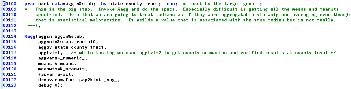
This is perhaps the most challenging step (not counting finding or creating the equivalency files) of the process. This is where we have to do the data allocation, apportioning the data based on the allocation factors from the equivalency files. But if you have a good tool set it can become very routine. We already discussed the %agg macro in our first case study. It won't change for this example. What makes it harder is having to specify those long lists of "mean" variables and their corresponding weights. But we already did this, taking advantage of the fact that we had a metadata set that make it pretty easy. We created global macro variables called _means and _meanwts with the values needed. So all we have to do is invoke the macro, specifying the parameters. As follows:
- The aggin parameter is where we tell it the data set containing the data to be aggregated. Note that this data set must contain all the variable specified in the aggby argument and must be sorted by those variables (not proc sort step, just above.)
- Aggout is where we tell the macro where to put the results, i.e. the aggregated data set.
- Aggby is where we specify the variables by which to aggregate the data. Since our county variable is 5-digit and includes the state, we would not have to include state here. But we like to keep it because we want it on the output set, and it also makes it easier to adapt this code to run against multiple states at once.
- Agglvl specifies how many levels of aggregation. The comment is important. While testing our code we specified a value of 2 for this parameter and then we got summaries at the county level as well as tract. We were able to look at the published county level data (it's in the usmcdcprofiles5yr data set we are using as our source here) and compare our allocated/aggregated data to see if our results matched. They did. This is always a good debugging strategy.
- Aggvars is a list of the variables to aggregate. We could have generated a specific list but it is easy enough to use the special SAS variable list _numeric_, meaning all variables that are of the numeric type. What allows us to do this is that we are very consistent in our archive data sets to always store codes as character variables.
- Means and meanwts have been discussed above. The great majority of the means variables are percentages.
- Facvar tells the program that it is to use the variable afact to apportion the data in the observation prior to aggregating.
- Dropvars just allows us to drop some variables we are not going to need. _nag_ is a special variable calculated by the macro to county the number of observations that were combined to form the output observation. We also no longer need the special equivalency file variables afact and pop2kint.
The run; statement is necessary (if running interactively) to cause the generated data step to actually run.
Post Step to add ID variables
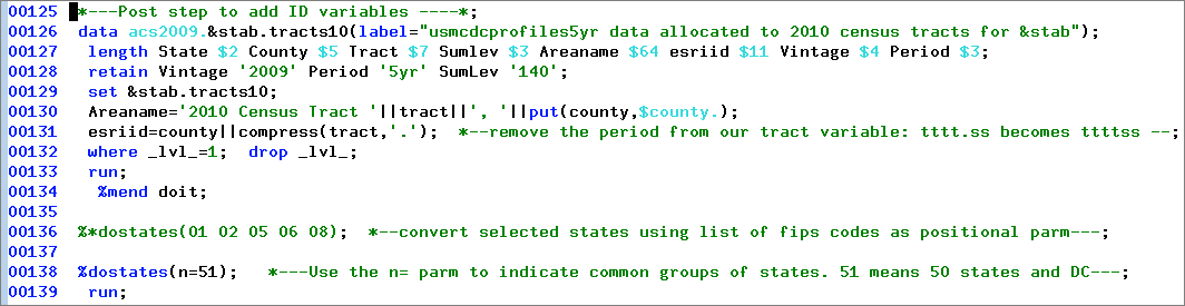
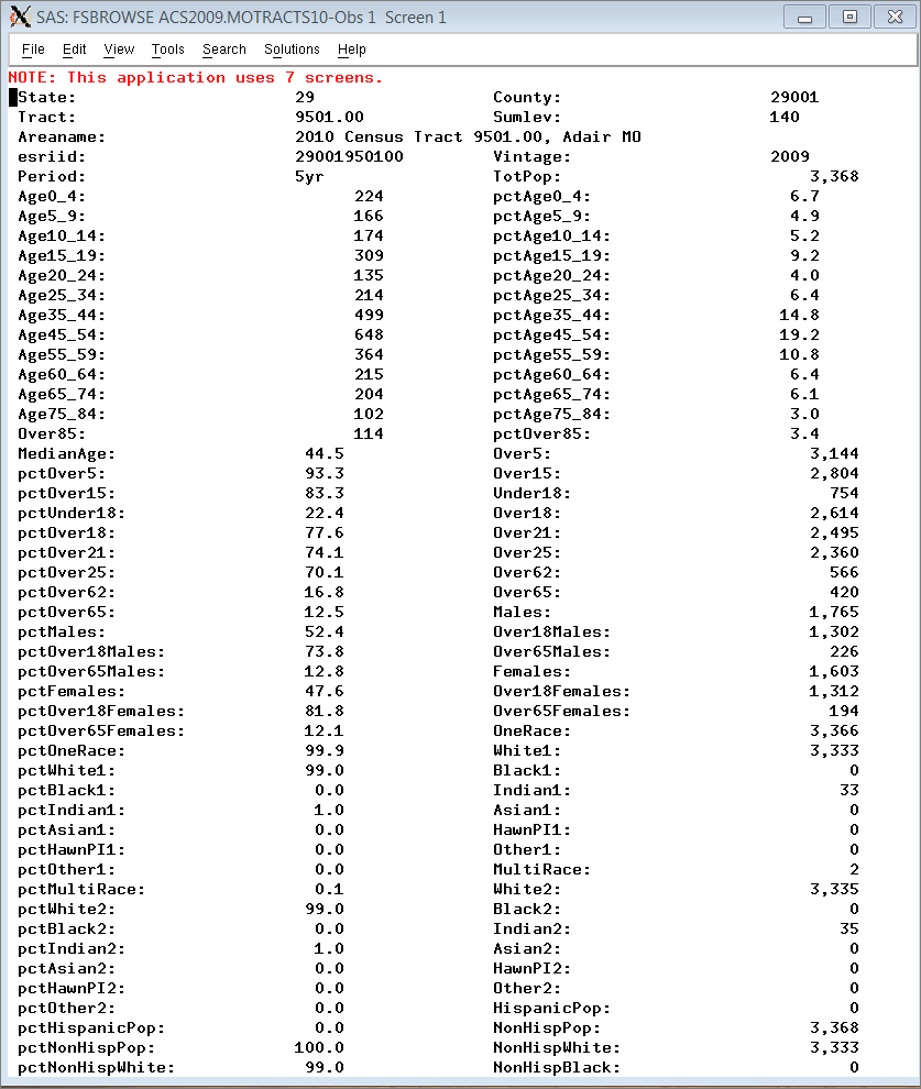
There is nothing too complicated here. We want to add some identifiers to make it easier for us and our Dexter users to be able to understand what these data are about. The ID variables Vintage, Period, and SumLev are constants and document the fact that these are vintage 2009 5-year period estimates at the census tract level. The Areaname variable is always helpful and starts with "2010" to emphasize that these are 2010 tracts (not 2000 versions such as are reported elsewhere in the acs2009 data directory). Tract is handy to have as a separate variable. The esriid variable corresponds to the portion of the Bureau's geoid variable without the first seven characters. For example, for the first tract in Adair county, MO partially displayed below, the value of Geoid would be 14000US29001950100, where the bold portion is the value of esriid.
Specifying these variables in a SAS length statement prior to the set statement causes them to be stored first within the observations on the SAS data set. This makes it easier to work with data extracted from the archive when all the IDs appear first. Here is a partial look at the first observation on the Missouri output data set:
Invoking the Macro for States
We use our %dostates utility macro in order to invoke the %doit macro for specified states. At line 136 you can see how we used it to run some test states by specifying their codes as the single positional parameter. This invocation has been commented out. Line 138 shows the other way to invoke %dostates using the n= parameter. We use n=51 to invoke the macro for all 50 states and DC.