Ten Things to Know about the American Community Survey
2005 Edition; revised April 2021
The American Community Survey (ACS) is a very important new source of data of the type usually associated with a decennial census, but based on survey data that are less than two years old. This list of items attempts to make users aware of some of the more important potential "gotcha"s that go with these data. NOTE: Much of this information is specific to the 2005 edition of the data and may not apply to data released in subsequent years. We have tried to avoid getting into statistical technicalities, but many of the items cited here are the result of statisticians doing things to reshape the data. In such cases, even if you cannot follow the details of why something might be the way that it is, at least know that the problem exists.
1. First, the good news.
The ACS data provides us with more information about our population and housing stock than we have ever had in our history outside of a decennial census year. The results of the survey have been tabulated in a very detailed fashion, with more than 1000 detailed ("base") tables, to go along with a series of custom profile, ranking, and subject tables, and geographic comparison tables summarizing the data for each available geographic area.
In addition to making the data itself readily available, the Bureau has also provided the usual access to excellent metadata and background information. There are even a series of online tutorials/Powerpoint presentations that provide excellent introductions to the data geared to new users. See the ACS home page for more info.
2. "Total population" is really "total population in households."
The 2005 survey did not include persons in group quarters (i.e., living in dormitories, nursing homes, prisons, military barracks, etc.). They were included for the 2006 data year and later. This limitation makes it difficult to cite any trend based on comparing 2000 decennial census data and the 2005 ACS data. The different survey universes used must always be taken into consideration. This limitation was not mentioned in table labels. The label says "Total Population" with the implicit qualification is "included in this year's sample universe".
3. Data from the 2005 ACS is only available for geographic areas with a total population of at least 65,000.
This somewhat arbitrary magic number is designed to avoid creating tables where the sample size would result in large standard errors (sampling error). Of course, many tables that are published in the ACS have universes well below the 65,000 threshold. Tables come with confidence interval sizes (MOE, for margin of error) to alert users to the reliability of the numbers. These MOE values are often quite large, especially when dealing with detailed subpopulations; just because an item gets published does not mean it can or should be used without noting the significant uncertainty involved.
In 2008, the Bureau began publishing tables for geographic areas of at least 20,000 population. These tables were based on combining the survey data for three consecutive calendar years (e.g. 2005 through 2007). In 2010, the Bureau began publishing tables for geographic areas of all sizes down to block groups based on data collected over the previous five calendar years (e.g., 2005 through 2009). These tables, based on multiple years of survey results, are commonly referred to as moving average tables. Note that for larger areas, you are able to choose from different sets of tables starting in 2008. The tradeoff will be between larger sample size vs. more current data.
4. The ACS is about characteristics of the population, not the size.
If you are looking forward to getting new and improved data regarding the number of Hispanics (or African-Americans, or foreign-born persons, or poor persons, etc.), don't get your hopes up. The ACS does not provide any new data regarding the counts of persons or households. This is because the Census Bureau does not weight ACS survey returns the way they do with decennial census surveys. In the decennial census, the Bureau assigns weights based upon their master address list, which is assumed to be definitive and complete. This is not the case with the MAF (master address file) used for the ACS. Although an initial weight may be assigned based on the number of households found in an area on the MAF, the person record weights are adjusted so that total population counts at the county level by certain age, race, gender, and Hispanic cohorts will match numbers published in the Bureau's detailed county-level demographic estimates. The result is that the number of cases (persons) in a table is really just a reflection of those estimates, and the data collected in the ACS simply controls the apportioning of those cases (total persons in households, households with Hispanic head, total males living in households, etc.) based on characteristics. So the ACS may tell us what portion of African-Americans are classified as living in poverty in a county, but the actual number of such persons is the result of applying that portion to the number of African-Americans that are estimated in the Bureau's estimates program. To make matters worse, the Bureau also adjusts the weights at the household level separate from the weights for persons.
5. Income as reported on the ACS is not compatible with income reported in the decennial census.
This is a surprising, rather frustrating, and unintended result that the Bureau does not yet fully understand. It has to do with how the questions regarding income are asked on the two survey instruments. The decennial survey asks a person about their income in the previous calendar year, whereas the ACS survey asks about income in the previous 12 months. Everything gets adjusted for inflation, but when the Bureau looks at test results, they have strong evidence indicating that income reported with the ACS version of the question is consistenly lower. See the Bureau's rather readable 16-page paper about this issue by Nelson, Welniak, and Posey. The official Bureau stance is that users should exercise caution when trying to do trend anlaysis regarding income or poverty measures using the decennial census vs. ACS data.
The income comparability problem is just one rather dramatic instance of an item being collected in the ACS that has issues of comparability with the same subject area as measured in the decennial census.
6. ACS tables contain suppressed data.
Users of decennial census data who have been around long enough to remember the problems with the 1970 and 1980 summary data sets because of data suppression will be disappointed to find out data suppression is back for the ACS. It happens at the base table level for the 1- and 3-year data products, but was not done for the 5-year data to be released for all geographic areas starting in 2010.
The Bureau applies what they refer to as their Data Release Rules to the base tables in order to protect us from tables whose reliability is unacceptable. Unfortunately, these rules suppress entire tables rather than just the unreliable cells within the tables (and, conversely, allow the publishing of very unreliable cells within tables whose overall reliabilty is deemed acceptable).
We do want to warn users about some of the unfortunate consequences of this approach by citing an example. Base table B17010 deals with the poverty status of families. It breaks the data down by type of family and presence of related children. The table has 41 cells in it. Many of these cells pertain to rather uncommonly-occurring categories such as "Non family, male-headed family households with no related children < 18". Because of this detail, and because the Bureau's algorithm for suppressing tables is designed to protect us from tables with small cell counts, this table winds up being suppressed for 4 of the 16 Missouri counties for which we have ACS data for 2005. The way this is supposed to work is that when a table is too detailed like this, then there will be a comparable C table with less detail. But there is no table C17010. So, you might think that at least we can go to the economic profile table (D03), which has an item telling us what percentage of all families in an area are below the poverty line. But it turns out that the Bureau does not go back to the original data to generate the profiles, but instead just derives/copies them from the base tables. This results in a missing value for the percent poor families item on the economic profile for Cape Girardeau county, MO. This, in spite of the fact that there are almost 19,000 family households in that county. And in the very same profile a poverty estimate appears for related children < 5 years, even though the number of children under 5 in the county is less than 4,000.
7. The ACS collects data for all 12 months of the year, not for just a single point in time.
The decennial census takes a snapshot of the population and housing stock based on a single day — April 1 of the decennial year. But ACS surveys are distributed year-round, so we have January data and December data. This can be a key factor in interpreting differences in data between the census and the ACS, especially so in areas that have seasonal populations, such as resort areas or college towns.
In the decennial census, you are counted where you are residing on April 1 (with a very few exceptions). With ACS it is more complicated; where you get counted is based on where you reside when you get the survey (unless you are only staying there temporarily, defined as less than two months). This should mean increased populations for places like Lake of the Ozarks (resort area with a large summer-only population) and lower populations for places like Lawrence, KS (college town, where most students are there on April 1 but not in the summer). However, since the population counts are then adjusted so that they sum to the numbers from the estimates program, maybe not. It may wind up affecting the characterstics (educational attainment goes down in Lawrence) without affecting the actual head counts.
8. Data products for the ACS are numerous.
They include:
- Base tables (aka "detailed tables") are the kinds of summary tables that users of decennial census summary files are used to. All the data in the other table types can be derived from the information in these tables. These tables have a naming scheme that consists of up to four parts. The first letter of the table ID is either a B or a C; a C table is a collapsed version of a B table with the corresponding table code. For example, tables B13008 and C13008 contain similar data: women who gave birth in the last year by marital status and foreign-born status. The more detailed B table provides a breakdown of the foreign born category by U.S. citizenship status. There will be instances when data will be suppressed in the B tables but will be available for the less-detailed C table. Each base table is identified by a five-digit number with leading zeroes, with the first two digits of the code corresponding to a topic. Some tables also have alpha suffixes as part of their IDs. Alpha suffix codes A through I are used to indicate that the table has a special race or Hispanic subpopulation. Thus, tables B05003 and B05003A contain similar data, but the former is a summary of the total population, while the latter is for the white-alone subpopulation. Additionally, a few tables have a "PR" suffix, indicating that they are specific to Puerto Rico. These will have the same root table ID as the corresponding table for U.S. geography. For example, tables B05001 and B05001PR have similar data, with the former available for all U.S. geographies and the latter just for Puerto Rico.
- Profile tables are special extracts based upon the base tables. These tables are much smaller and are used to provide good overviews of an area. There are four of them: DP01 — general demographic summary (age, sex, race, hispanic, etc.); DP02 — social profile (education, merital status, fertility, etc.); DP03 — economic profile (income, poverty status, employment status, etc.); and DP04 — housing profile (housing values, tenure, units in structure, etc.).
- PUMS files for users who want to "roll their own" data tables/analyses (see below).
The 2005 data products were released in waves over the late summer and early fall of 2006. As of mid-September, waves 1 and 2 had been released, covering subjects in the first three DP categories. The housing data were released the first week of October; the narrative profile data products along with some more detailed data regarding population subgroups were due in November.
9. PUMS data included in ACS products.
The public use microdata sample (PUMS) data allows users to access a 1% sample of ACS surveys. This represents about 40% of the available data, since the overall ACS sample is about 1-in-40 or 2.5% of all households within a given year. Researchers who are comfortable with the statistical aspects of analyzing such data (typically with a commercial statistical software package such as SAS or SPSS) can create their own custom tables. The smallest unit of geogrpaphy on these files is the PUMA (public use microdata area) — the same units identified on the 2000 Census PUMS files. Care must be taken when using PUMS files because of the small sample size.
The MCDC has a complete collection of the ACS PUMS data, which is kept in its own separate data directory called acspums. This directory contains such files for multiple years.
10. The PUMA (public use microdata area) level geography lets you map and analyze data for your entire state.
One of the things people do with census data is creating thematic maps or summary reports that show spatial distributions of data within their state or region. This sort of thing is not generally doable with the ACS data because of the limited geography available (as of 2005). There are two levels of geography where the 2005 data at these levels is available for all areas, covering the state; they are congressional districts and PUMAs. The former tend to be too large for mapping purposes, while the latter are considerably smaller and hence better suited for a mapping application.
Users who are not familiar with PUMAs may find it worth their while to become more familiar. To learn more, you can start with a set of PDF base maps accessible from the Bureau's web site. When you get to the PDF document, note that the first page is an index page that displays entities called super PUMAs. These are not the PUMAs you want. The PUMAs you do want are sometimes referred to as 5% PUMAs, because they were the geography used on the 5% sample PUMS files in 2000, whereas the super PUMAs (also known as 1% PUMAs) were the ones used on the 1% PUMS files in 2000. The key to using these maps is to understand that the 5% PUMAs nest within the super PUMAs, and these PDF files have one or more inset maps showing more detail for metropolitan areas within the state, and then one page for each super PUMA showing the boundaries of the 5% PUMAs. The maps also show relevant place and county boundaries to help you see what geographic areas correspond to the PUMAs.
A more precise and easy way of seeing the relationships of PUMAs to other geographic entities, such as counties, is using one of the MCDC's Geocorr web applications. For example, we invoked the application and specified that we wanted:
- Colorado as the state to process
- PUMA for 5% Samples (2000) as the source geography
- County (2000) as the target geography
- Generate 2nd allocation factor (AFACT2) selected
Try replicating these specs yourself. You should get a pair of output files, one a CSV file that can be used for importing to an Excel, and the other a report file (text or HTML). Here is what you should see on the first few lines of that report:
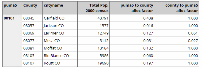
Each line represents the intersection of the 00101 PUMA with a Colorado county. The 4th column shows the 2000 census pop count for the intersection (the portion of the county within the PUMA), and is followed by 2 columns of allocation factors. The first allocation factor says what portion of the PUMA's total population is in the County (43.8% of persons living in PUMA 00101 also live in Garfield county), while the second indicates what portion of the county's population also reside in the PUMA (100% of Garfield county resideents live in PUMA 00101, and only about 5% of Larimer countians reside in that PUMA).
For more information regarding PUMA geography see the MCDC's page describing PUMAs in considerable detail, including a link to a custom report that shows all the 2000 PUMA codes in the U.S. along with their Super PUMAs and what counties and major cities are contained within each.