MCDC News and Updates

ACS 2016-2020 five-year data release is delayed until March 2022

The U.S. Census Bureau announced on Nov. 10 that the American Community Survey (ACS) 2016-2020 five-year data release will be delayed until March 2022. The ACS normally releases its five-year data products in December of every year. However, according to the Bureau’s statement, “Additional time is needed to continue refining our methodology so that we can minimize the impact of nonresponse bias due to the COVID-19 pandemic.”

This delay will affect several of MCDC’s data applications, notably ACS Profiles, Circular Area Profiles (CAPS ACS), and Missouri County Fact Sheets.

Expect additional updates regarding this matter in December.


ACS 2015-2019 5-year Data Is Here

We now have the 5-year ACS 2015-2019 data available on our website. The ACS Profiles and ACS Trends applications include the new data.

Both profiles and base tables (aka summary or detailed tables) are also available in SAS/Dexter format in our data archive at acs2019.

Please let us know if you encounter any issues with the data.

We’ve also made numerous small updates to our data applications and website.

Map of the Month

Missouri Educational Attainment and Income

Educational attainment is an established, validated predictor of income. This map-of-the-month series looks at the distribution of both characteristics in Missouri’s counties. Derived from the U.S. Census Bureau, American Community Survey (ACS) 2012-2016 5-year data, Missouri households are mapped here by level of educational attainment and median household income, while a bivariate choropleth map displays the variable impact of earning less than a high school diploma on household income.

Education vs. Income in Missouri, 2012-2016

The bar chart, based on the 2016 ACS 1-year release, establishes the relative distribution of median household income by level of education. While the overall median household in Missouri realizes approximately $36,000 in income, the median household in Missouri headed by someone without a high school diploma or GED is closer to $20,000.  Completing high school results in a bump of roughly  $10,000, with the median household income of high school graduates a little more than $30,000. Completing some college or an associate’s (2-year degree) results in an incremental increase in household median income to the mid-$30,000 range, but it is completion of a bachelor’s degree or greater that accelerates median household income into the mid-$40,000 to mid-$50,000 range annually.

Educational attainment, however, is not the only driver of income. Access to workforce opportunities and proximity to infrastructure impacts potential income too. Review of the Median household income map reveals the influence of infrastructure investment and population density in driving up wages and income, as seen in the counties shaded in the darkest green.  It’s also interesting to visually note the geographically layered gradation of quantiles of the state with the I-70 highway corridor connecting Missouri’s relatively high income metropolitan areas, and the agricultural northern tier of counties falling into the mid-quantiles, while lower income households concentrate in the southern tier of counties (with exception of income concentrating in the Springfield metro area).

Not surprisingly, a close look at the concentrations of level of educational attainment (the blue-scale maps), correlate at the county level to the median household income map fairly predictably: Populations with higher concentrations of higher levels of education also have higher median household incomes.

The bivariate choropleth map, Median household income by percent of adults with less than high school diploma or GED, lets us see the outliers as well as validating the correlations we anticipated. For example, the truer the shade of blue a county is coded, the higher the percent of the adult population without a high school diploma/GED and the higher median household income indicating some combination of higher wage job and income opportunities relative to educational qualifications. We see these on the periphery of the other end of the spectrum, counties with higher median household incomes and the lowest rates of households with low educational attainment, suggesting “bedroom” communities. Further study to confirm this pattern might include looking at patterns of in-migration over time and commuting patterns.


New American Community Survey Data Released for 2013

The 2013 American Community Survey (ACS), released today in its one-year version, provides a multitude of statistics that measure the social, economic and housing conditions of U.S. states, counties, and communities. More than 40 topics are available with today’s release, such as educational attainment, housing, employment, commuting, language spoken at home, nativity, ancestry and selected monthly homeowner costs.

The ACS gives communities the current information they need to plan investments and services. Retailers, homebuilders, police departments, and town and city planners are among the many private- and public-sector decision makers who count on these annual results.

“The American Community Survey is our country’s only source of small area estimates for social and demographic characteristics,” Census Bureau Director John H. Thompson said. “As such, it is indispensable to our economic competitiveness and used by businesses, local governments and anyone in need of trusted, timely, detailed data.”

Also released today are two reports providing analysis on income and poverty for states and large metropolitan areas. The ACS three- and five-year data for 2013 will be released in October and December of this year, respectively.

Following are some highlights of the new ACS 2013 one-year release and related reports.

Income

  • For 2013, median household incomes were lower than the U.S. median ($52,250) in 28 states and higher in 19 states and D.C. (Three states did not have a statistically significant difference from the U.S. as a whole.)
  • In 2013, the states with the highest median household incomes were Maryland ($72,483) and Alaska ($72,237). Mississippi had the lowest ($37,963).
  • Median household income among the 25 most populous metro areas was highest in the Washington, D.C. ($90,149), San Francisco ($79,624), and Boston ($72,907) metro areas.

Income Inequality

Household Income: 2013 examined the Gini index for states and large metro areas. The Gini index is a summary measure of income inequality, ranging from 0 (complete equality) to 1 (complete inequality). Among the findings:

  • Five states and D.C. had Gini indexes higher than the U.S. index of .481; 36 states had lower Gini indexes than the U.S.
  • The Gini index of 15 states increased from 2012 to 2013. Alaska was the only state to have a decrease. All other states saw no significant change.
  • The highest Gini index was in the District of Columbia (0.532). Alaska’s (0.408) was among the lowest.
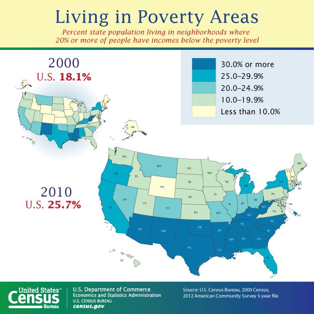
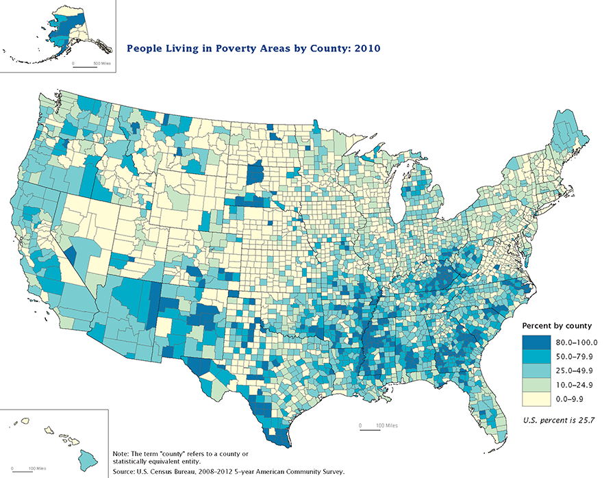
Poverty

  • Two states — New Hampshire and Wyoming — saw a decline in both the number and percentage of people in poverty. New Hampshire’s poverty rate declined from 10% in 2012 to 8.7% in 2013. Wyoming’s rate declined from 12.6% to 10.9%.
  • Three states saw increases in both the number and percentage of people in poverty between 2012 and 2013. New Jersey’s poverty rate increased from 10.8% in 2012 to 11.4% in 2013; New Mexico increased from 20.8% to 21.9%, and Washington increased from 13.5% to 14.1%.
  • In 2013, Mississippi had the highest poverty rate among states (24%), followed by New Mexico (21.9%). Both states also had the highest percentage of the population below 125% of the poverty level: 30.3% in Mississippi and 28.3% in New Mexico. About one in 10 people in both states had incomes less than 50% of the poverty level.
  • Among large metropolitan areas, one of the lowest proportions of people with incomes less than 50% of the poverty level in 2013 was 4.2% in the Washington, D.C., metro area, while one of the highest proportions was 8.4% in the Phoenix metro area.

Health Insurance

  • Between 2012 and 2013, 13 states and Puerto Rico saw a statistically significant increase in the percentage of civilians covered by health insurance. Two states (Maine and New Jersey) saw a decrease.
  • Among people whose incomes were below 138% of the poverty threshold, 25.6% were uninsured in 2013. (Under the Affordable Care Act, states have the option of expanding Medicaid eligibility to those with incomes at or below 138% of the poverty threshold.) Among people whose incomes were at or above 200% of the poverty threshold, 9.2% were uninsured in 2013.
  • Among the top 25 largest U.S. metropolitan areas, the uninsured rates were highest in Miami (24.8%), Houston (22.8%), and Dallas (21.5%) and lowest in Boston (4.2%), Pittsburgh (7.5%), Minneapolis (8.1%), and Baltimore (8.7%).
  • Among the top 25 large metropolitan areas, Tampa, Detroit, and Riverside, Calif., had public coverage rates of 33% or higher.

Computer and Internet Access

The 2013 American Community Survey included new questions to produce statistics on computer and Internet access. Mandated by the 2008 Broadband Data Improvement Act, the data will help the Federal Communications Commission measure broadband access nationwide. The data will also help identify communities eligible for available grants to expand access.

Some findings: 83.8% of the nation’s households have a computer (either desktop, laptop, tablet or smartphone). 74.4% have some form of Internet access at home. The Census Bureau is releasing a more detailed report on the new findings in early October.

ACS Report

One Quarter of U.S. Residents Live in Poverty Areas

A new report from the U.S. Census Bureau’s American Community Survey (ACS) shows that one in four U.S. residents now live in poverty areas — up from fewer than one in five in 2000.

A “poverty area” is defined as any census tract with a poverty rate of 20% or more.

The number of people living in poverty areas increased from 49.5 million (18.0%) in 2000 to 77.4 million (25.7%) in 2008-2012. The overall U.S. poverty rate was 14.9% for the same period.

Percent living in poverty areas by state, 2010

By state, the percentage of people living in a poverty area ranged from 6.8% in New Hampshire to 48.5% in Mississippi. Several states saw declines over the period: District of Columbia (-6.7%), Louisiana (-3.6%), West Virginia (-2.3%), Alaska (-0.4%), Hawaii (-1.0%), and Alaska (-0.4%). On the other hand, North Carolina (17.9%), Oregon (16.0%), Tennessee (16.0%), Arkansas (15.7%), and Georgia (14.6%) had the largest increases in the proportion of people living in poverty areas.

More than half of people living in poverty lived in a poverty area, and about 30% of people living in poverty areas had incomes below the poverty level.

The report, Changes in Areas with Concentrated Poverty: 2000 to 2010, uses data from the 2000 Census and the 2008-2012 ACS five-year estimates to analyze changes in the spatial distribution and socioeconomic characteristics of people living in poverty areas.

According to the report’s author, Alemayehu Bishaw of the Census Bureau’s Poverty Statistics Branch: “Researchers have found that living in poor neighborhoods adds burdens to low-income families, such as poor housing conditions and fewer job opportunities. Many federal and local government agencies use the Census Bureau’s definition of poverty areas to provide much-needed resources to communities with a large concentration of people in poverty.”

People living in poverty areas by county, 2010

Other highlights of the report:

  • Missouri’s percentage of people living in poverty areas (24.9%) is just slightly lower than the national rate and represents a change of 9.9% over the period.
  • In the 2008-2012 period, in 14 states and D.C., 30% or more of the population lived in poverty areas. In 2000, this was true of four states and D.C.
  • Of the people living in poverty areas in the 2008-2012 period, 51.1% lived in central cities of metro areas, 28.6% in suburbs and 20.4% outside metro areas.
  • Many of the counties with 80% or more of the population living in poverty areas were clustered in and around American Indian reservations (in New Mexico, Arizona, South Dakota, and North Dakota) or in the Mississippi Delta region (including portions of Mississippi, Louisiana, and Arkansas).
  • About 38% of all families headed by a female householder with no husband present lived in a poverty area — the largest proportion among all family types.
  • Blacks, American Indians and Alaska Natives, and those in the “some other race” category were the race groups most likely to live in poverty areas, at 50.4%, 47.8%, and 48.3%, respectively. Whites, however, experienced the largest increase in the proportion living in poverty areas, from 11.3% in 2000 to 20.3% in 2008-2012.
  • Employed people saw a larger increase (8.0%) than the unemployed (3.4%) in people living in poverty areas over this period.
  • The Midwest region experienced the largest increase over the period (9.8%).